Multi-Layer Perceptron

This post covers the history of Deep Learning, from the Perceptron to the Multi-Layer Perceptron Network.

1. Perceptron

Key idea (1958, Frank Rosenblatt)

1. Data are represented as vectors
2. Collect training data: some are positive examples, some are negative examples
3. Training: find $a$ and $b$ so that
   • $a > x + b$ is positive for positive samples $x$
   • $a > x + b$ is negative for negative samples $x$
4. Testing: the perceptron can now classify new examples.

Notes:

• This is not always possible to satisfy for all the samples
• Intuitively, it is equivalent to finding a separating hyperplane

Training the perceptron: At the time, ad hoc algorithm:

1. Start from a random initialization
2. For each training sample $x$:
   • compare the value of $a > x + b$ and its expected sign
   • adapt a and b to get a better value for $a > x + b$

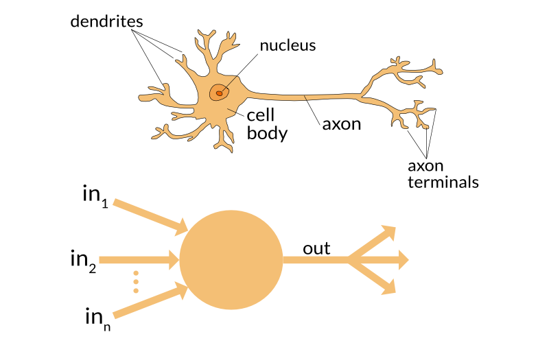
Note: The perceptron is roughly inspired from the neuron:

Limitations: 1969, Perceptrons book, Minsky and Papert

• A perceptron can only classify data points that are linearly separable:
• Fail easy case such as the x-or function

Consequence: It is seen by many as a justification to stop research on perceptrons and entails the “AI winter” of the 1970s.

2. Multilayer Perceptron/Neural Network

Key idea (1980 - Rumelhart, Hinton, Williams) “Chain” several perceptron together at different depth, with the help of a “squashing” function.

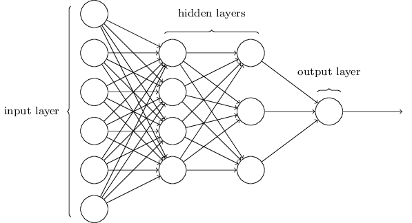
Formalism:

1. Input layer: $x$ is the same vector used for the perceptron.
2. Hidden layer: consists of perceptrons + squashing function
   • Perceptrons weight their input $Wx + b$, where $W \in \mathbb{R}^{perceptrons\times features}$
   • Squashing / activation function $h = g(Wx+b)$ “rescales” the input for the next layer.
3. Output: $y = W_{2}h+b_{2}$

Note: We can construct networks with arbitrary number of hidden layers, hence the usefullness of the activation function.

We can find $W, b, W_{2}$, and $b_{2}$ with the objective:

where $\mathcal{T}$ is the training set (features $x$ and expected output $d$).

Note: A Multilayer Perceptron solves non-linearly separable problems such as the x-or function with $g(a) = max(a, 0)$

In practice:

• Do NOT use a least-squares loss function for classification problems!
• There are no closed-form solution so we use gradient descent.

3. The Topology of the Functions Learned by Feedforward Networks

Universal Approximation Theorem Hornik et al, 1989; Cybenko, 1989

Any continuous function can be approximated by a two-layer network (with ReLU activation).

The function learned by a Deep Neural Network with the ReLU operator is:

• Piecewise affine
• Continuous
• Equations of the final regions are correlated, in a complex way