Linear Regression

In layman terms, a Linear Regression consists in predicting a continuous dependent variable $Y$ as a linear combination of the independent variables $X = {x_{1}, …, x_{n} }$. The contribution of each variable $x_{i}$ is expressed by a parameter $\beta_{i}$. Altogether, it is a simple weighted sum:

where $\beta$ are the parameters, also called weights. It should be noted that in the above formula, the sum begins at $i = 0$ to incorporate the intercept (i.e. the constant term). As for the parameters, they are learned to minimize the quadratic loss function:

The parameters we consider best are the one that minimizes this error.

1. Least Mean Squares

TL; DR: We use gradient descent:

where $\alpha$ is called the learning rate. Simplifying leads to this:

Least Mean Square update rule (single training example): $\beta_{j} := \beta_{j} + \alpha (y^{(i)} - h_{beta}(x^{(i)})x_{j}^{(i)}$

Batch gradient descent:

It does not scale well with the number of famles $m$.

Stochastic Gradient Descent:

Less costly than Batch Gradient Descent $\Rightarrow$ Faster to get near the minimum.

Results:

• The magnitude of the update is proportional to the error term.
• J is a convex quadratic function $\Rightarrow$ gradient descent always converges.

2. Closed form solution - Normal equations

There is a way to solve this with Linear Algebra by reformulating the loss:

where $X \in \mathbb{R}^{n\times m}$ is our $n$ samples with $m$ features.

By setting the derivative of $J(\beta)$ to $0$ and solving the problem with matrix derivatives, we obtain:

Result / Definition (Ordinary Least Square estimate):

3. Regularization

3.1. Least Absolute Shrinkage and Selection Operator (LASSO)

To enhance both the prediction accuracy model and the interpretabiliy of the produced model, LASSO alters the fitting process by selecting a subset of the provided covariates for use in the final model. To this effect, it shrinks the OLS coffcient toward zero (with some exactly set to zero).

Definition (LASSO estimate): $\hat{\beta}_{lambda} = \text{argmin}_{\beta} J(\beta) + \lambda \sum_{j=1}^{p}\mid \beta_{j} \mid$

Terminology ($\mathcal{l}_{1}$ penalty): This is the righmost term of the above equation.

Note: One can proove that this is equivalent to:

where

is a bijective application.

3.2. Ridge Regression

Ridge Regression is also a regularization technique, with however possess a different penalty term, that prevents it to perform variable selection in most cases.

Definition (Ridge Regression estimate): $\hat{\beta}_{lambda} = \text{argmin}_{\beta} J(\beta) + \lambda \sum_{j=1}^{p}\beta_{j}^{2}$

The difference with LASSO regularization resides in the penalty term, which is in this case a $l_{2}$-penalty.

Similarly to LASSO, there exists a bijective application $s_{\lambda}$ that states the equivalent form (optimization problem):

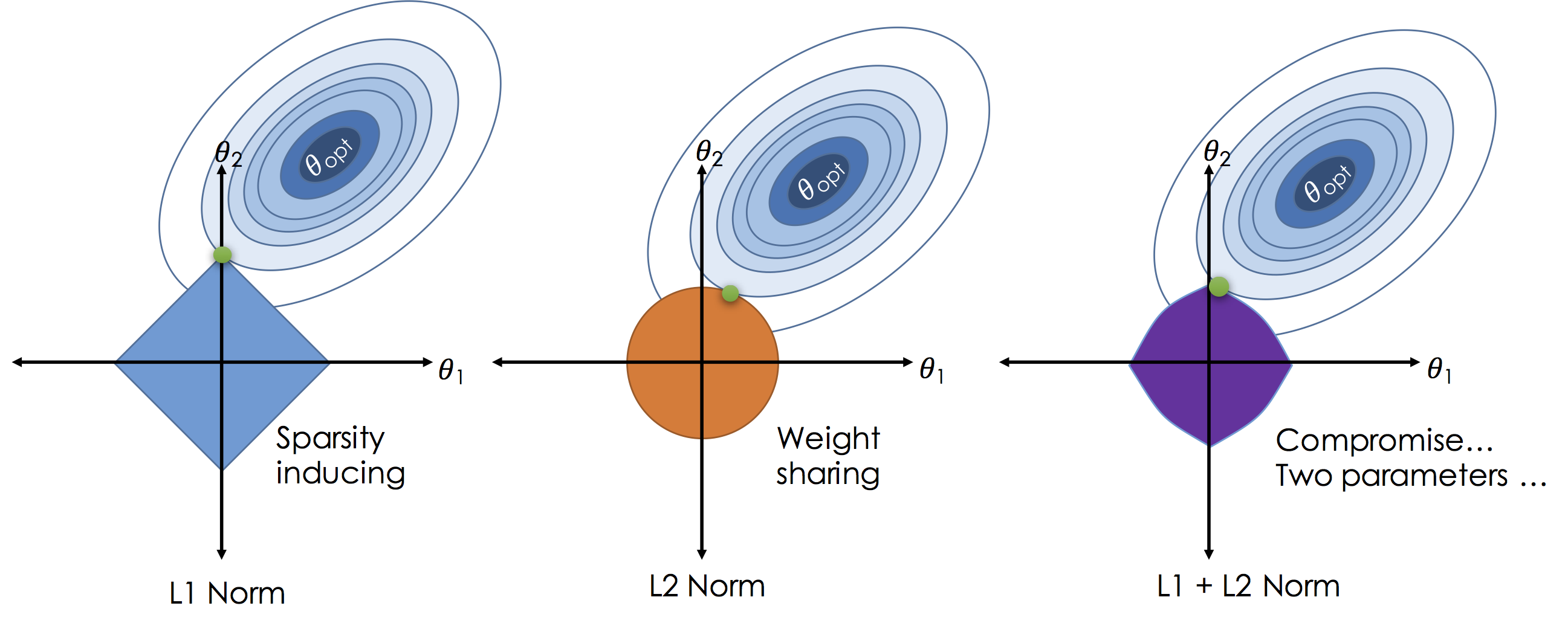
3.3. Geometric intuition (p = 2)

The optimization problems defined for both the LASSO and the Ridge Regression shrinkages yield an geometric explanation of those two shrinkage methods:

where the blue areas are the constraint region and the red lines the contours of the RSS.

Both LASSO and Ridge Regression estimates are defined by the intersecion ot the RSS lines and the constraint region. It is why variable selection is induced by the LASSO as the sharp corners of the constraint area are more likely to intersect the RSS lines. When $p > 2$, the variable selection holds due to the constraint polytope sharp corners.

3.4. Extensions to Elastic Nets

The LASSO penalty is somewhat indifferent to the choice among a set of strong but correlated variables. The ridge penalty, on the other hand, tends to shrink the coefficients of correlated variables toward each other.

Elastic Net is a hybrid approach that blends both penalization of the $l_{1}$ and $l_{2}$ norms. Formally, it is a convex combination of both, as it minimizes the following:

where $\alpha \in [0, 1]$ is a hyper-parameter controlling how much of $l_{1}$ or $l_{2}$ penalization is used.

Comparing to LASSO and Ridge Regression, an instance of elastic net yields the following constraint region for p=2

Note: LASSO tends to select noisy predictors with a high probability, leading to an inconsistent variable selection.

4. Locally weighted Linear Regression

TL; DR: The idea is to weight every training sample sample error according to their distance to the point $x$ we wish to predict. Precisely:

Weights choice (Gaussian kernel) $w^{(i)} = exp(-\frac{(x^{i}-x)^{2}}{2\tau^{2}})$

The space of functions $\mathcal{H}$ corresponding to the Gaussian kernel turn out to be very smooth. Therefore, a learned function (e.g, a regression function, principal components in RKHS as in kernel PCA) is very smooth. Usually smoothness assumption is sensible for most datasets we want to tackle.More here

Parameteric vs. Non-parametric Algorithms described above are parametric (have fixed, finite number of parameters), which are fit to the data. Once fitted, we no longer need to keep the training data to make future predictions.

For locally weighted linear regression, we need to keep the entire training set around. The term “non-parametric” (roughly) refers to the fact that the amount of stuff we need to keep in order to represent the hypothesis h grows linearly with the size of the training set.

5. Good practices

1. Make a significance test ($t$-test) $H_{0}:\{\beta_{i}=0 \} \text{ vs } H_{1}:\{\beta_{i}=0\} \$
2. Multicollinearity diagnostic (compute $det(X^{T}X)$, Variance Inflation Factors)
3. Check for eventuals transformations of the response (BoxCox method, typically $x \mapsto log(x)$)
4. Make a thorough residual analysis
   • Residual plot of fitted values: Externally studentized residuals
   • Normal probability plot

5. Leverage and influential points analysis (plot hat values)

   • Hat matrix diagonal: is a standardized measure of the distance of the $i$-th observation from the centroïd of the $X$ space. Therefore, large hat values ($h \geq \frac{2m}{n}$) reveal observations that are potentially influential because they are remote in $X$ space from the rest of the sample.

   • Cook’s distance: of the $i$-th point is a measure of the squared distance between the least-squares estimate based on all points and the estimate obtained by deleting the i-th point.
     • $D_{i}$ combines residual magnitude for the $i$th observation and the location of that point in $X$ space to assess influence.
     • $D_{i} > \frac{4}{n-m-1}$ typically indicates influential points.
   • CovRatio measure provide informations about the precision of estimations, which is not conveyed by the previous quantities.

https://math.stackexchange.com/questions/2624986/the-meaning-behind-xtx-1 https://www.quora.com/How-would-linear-regression-be-described-and-explained-in-laymans-terms