
Introduction to reinfocement learning
Mis à jour :
Reinforcement learning find its roots in several scientific fields, such as Deep learning, Psychology, Control, Statistics (but not limited to!). It typically consists of taking suitable action to maximize reward in a particular situation. Below is a common illustration of its core idea:
:max_bytes(150000):strip_icc()/2794863-operant-conditioning-a21-5b242abe8e1b6e0036fafff6.png)
Supervised vs Evaluative Learning
Supervised learning paradigm reach its limit when it comes to improve upon the performance of the traning data (a supervised learning task trained with the best chess player will not be better at chess than the best player).
The main difference between supervised learning and reinforcement learning is whether the feedback received is evaluative or instructive.
Instructive feedback tells you how to achieve your goal, while evaluative feedback tells you how well you achieved your goal.
Supervised learning solves problems based on instructive feedback, and reinforcement learning solves them based on evaluative feedback.
ADD TABLE
Framework
The typical formalization of reinforcement learning problems is based on the concepts of agent evolving in an environment, as described in the following diagram:
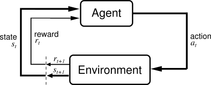
where an agent acts via a policy $\pi(s, a)$ on an environment, which in turn emits bach a reward $r(s, a)$ and a new state $s’$ (or an observation) to the agent. It should be noted that the behavior of both the environment and the agent is usually Markovian (details below).
Notes:
- Partial observation of the environment leads to partially observable Markov Devision Processes
- The interaction with the environment are usually divided into discrete episodes
- The environment can depend on a history of previous states
Reward hypthesis
Each action $a$ allows to potentially obtain a reward so we are fundamentally interested to $r(s, a)$ for a given state $s$.
Assumption: All goals can be described by the maximisation of the expected cumulative reward.
Ex.: Score in a game. Ex. 2: Typical image classification is not a RL task EXAMPLE
Taxonomy of Reinforcement Learning
Altough the previously discussed framework remains relatively unchanged accross RL problems, the goals and settings of the problems differ.
What is the goal?
- Control: Determining an optimal policy
- Evaluation: Evaluating a policy
Is a model supporting the problem?
- Model free: No model of the environment is learned / used and is instead planned directly from experience. (-> No speficic assumpion)
- Model based: Attempt to learn / exploit a model of the environment with the goal of using the model (models can vary in terms of efficience in design and speed)
Should we encourage discovery of the problem or reward optimization?
- Exploration: The agent discover new states, eventually making mistakes.
- Exploitation: The agent optimises its cumulated reward with the knowledge of prior discovery.
- Fundamental trade-off: Similarly to the bias-variance tradeoff in conventional Machine Learning, the agent needs to balance both exploration and exploitation phases to produce meaningful policies and avoid suboptimal results.
Mathematical formalization
States / Actions
States: We refer to a state $s$ as an element from $\mathcal{S}$ a countable set:
Examples:
- Successive rounds of Tic Tac Toe.
- Successive chess plays
Actions: We refer to an action a as an element from $\mathcal{A}$ a countable set.
Examples:
- Nought or cross
- Legal chess moves
State-action transitions
To understand in-depth the incoming Mathematical concepts, the reader should be familiar with Markov Random Processes.
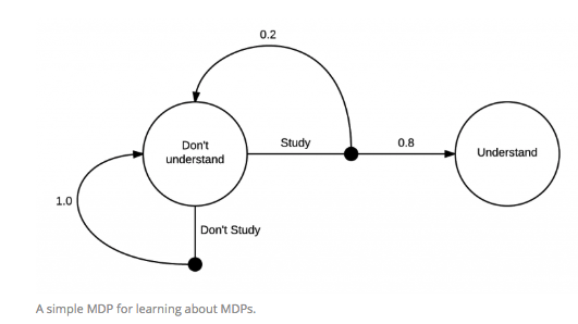
In a nutshell, a Markov Decision Process (MDP) is a 4-plet $(\mathcal{S}, \mathcal{A}, p, \gamma)$ where:
- $\mathcal{S}$ is a discrete set of states
- $\mathcal{A}$ is a discrete set of actions
- $p$ is a discrete probability transition kernel
- $\gamma$ is a discount factor that (similar to money value in finance)
The transition kernel models the probability to fo from a state $s \in \mathcal{S}$ with action $a \in \mathcal{A}$ to the state ${s’}\in \mathcal{P}(\mathcal{S})$ and reward ${r}\in \mathcal{P}(\mathcal{A})$. In terms of notation, the evaluation of this function will be denoted:
Two important results can be derived from the above defined kernel, namely:
- Probability measure: $p(. \mid (s, a)) \text{, } \forall (s, a) \in (\mathcal{S} \times \mathcal{A})$
- Next state probability: The expression below qualifies the probability of $s’$ realization under the policy $(s, a)$, noted as $s\mapsto^{a} s’$:
Reward function
Let $(S, A)$ a state-action pair. Then, the next state $S’$ as well as the corresponding reward $R$ are given by:
where $\mathcal{U}$ is the borel set. Now that these probabilities are properly defined, we can naturally express the reward function as:
Cumulative reward: For a given $\gamma \in ]0, 1]$ and a sequence of rewards $R_{1}, …, R_{n}$ we define the return (cumulative reward) as:
which will prove useful in discounting intermediate rewards later on.
Policy
We are interested in designing a policy which dictates to an agent what action to take given a particular state. It should be noted that the definition of the policies vary with the context (see tables below)
| Deterministic | Stochastic | |
|---|---|---|
| Stationary | $\pi = (\pi_{1}, \pi_{1}, …)$, with $\pi_{i}:\mathcal{S}\mapsto \mathcal{A}$ | $\pi = (\pi_{1}, \pi_{1}, …)$, with $\pi_{i}:\mathcal{S} \times \mathcal{A} \mapsto \mathbb{R}_{+}$ |
| Non-stationary | $\pi = (\pi_{1}, \pi_{2}, …)$, with $\pi_{i}:\mathcal{S}\mapsto \mathcal{A}$ | $\pi = (\pi_{1}, \pi_{2}, …)$, with $\pi_{i}:\mathcal{S} \times \mathcal{A} \mapsto \mathbb{R}_{+}$ |
Note: The stochastic case $\pi_{i}:\mathcal{S} \times \mathcal{A} \mapsto \mathbb{R}{+}$ verifies $\sum{a} \pi(a\mid s) = 1$
Interaction of the agent given a policy: Given a policy, one can define a Markov chain via:
At each step $n$, the agent is at the state $S_{n}$ and following its policy $\pi$, performs the action $A_{n} = \pi(S_{n})$ reaches:
Then, an episode is a sequence $S_{0}, A_{0}, R_{1}, S_{1}, A_{1}, R_{2}, S_{2}, A_{2}$
State value function
In a stationary setting, the value function $v^{\pi}:\mathcal{S}\mapsto \mathbb{R}$ (of a state $s$) is the expected reward if you start at that state and continue to follow the policy $\pi$.
As for the meaning of the expectation $E_{\pi}$ under a policy $\pi$ and an initial distribution $\mu$ on the state, we write:
where $p(s’\mid s) = \sum_{a}p(s’, a, s)\pi(a\mid s)$.
Key idea: The expectation in that formula is over all the possible routes starting from state $s$. Usually, the routes or paths are decomposed into multiple steps, which are used to train value estimators. These steps can be represented by the tuple $(s,a,r,s′)$ (state, action, reward, next state)
Note: Even if the policy is deterministic, the reward function and the environment might not be. Nor the value function is not deterministic.
Optimal value function: A policy $\pi^{*}$ is called optimal if:
Bellman equation
The Bellman equation is a necessary condition for the optimality associated with dynamic programming. It writes the value of a decision problem at a certain point in time in terms of the payoff from some initial choices and the value of the remaining decision problem that results from those initial choices. This breaks a dynamic optimization problem into a sequence of simpler subproblems, as Bellman’s “principle of optimality” prescribes.[2]
It means Q-value(state) = reward + the discounted Q-value(state) easily reachable from state.
we can transform the value function into:
Under the assumpion that $\gamma < 1$ and $\mid\mid\mathcal{P}^{\pi}\mid\mid\leq 1$ we obtain:
Implementation notes:
- The formula $(I-A)^{-1} = \sum_{k\geq 0} A^{k}$ is useful for inverse approximations.
Sources:
https://stats.stackexc https://joshgreaves.com/reinforcement-learning/introduction-to-reinforcement-learning/ ——
Laisser un commentaire