
Low-level vision framework
Mis à jour :
The problem of image analysis and understanding has gained high prominence over the last decade, and has emerged at forefront of signal and image processing research (read more here). In consequence, my first post on computer vision will deal with the basics of image understand.
These notes aim to provide a Mathematical framework for the model of images. Specifically, they review the use of basic operators such as convolutions, correlation and cross-correlation in signal processing.
Then, we will define two approaches for expressing an image into a desirable signal:
- Spatial basis is suited for pixel like input and is built upon the Dirac Delta delta function.
- Frequency basis is based on the 2D Fourier transform.
This framework is motivated by the fact that images are finite and with compact support, so they behave well mathematically and most properties hold for them.
1. Mathematical reminder - the 1D case
In this section, we will review some mathematical concepts (convolution-like operations, $L_{2}$ space) and we will see why we can restrict ourselves to a discrete context.
1.1. Convolution, correlation, autocorrelation
Three common problems in signal processing are important enough to motivate this reminder:
1.1.1. For an input signal $f$, what is the output of a filter with impulse response $g(t)$?
The answer is given by the convolution $f(t) * g(t)$. Mathematically, the convolution is an operation on two functions $f$ and $g$ which produce a third function $f * g$ that expresses how the shape of one is modified by the other.
1.1.2. Given a noisy signal $f(t)$, is the signal $g(t)$ somehow present in $f(t)$?
In other words, is $f(t)$ of the form $g(t)+n(t)$, with $n(t)$ is noise? The answer can be found by the correlation of $f(t)$ and $g(t)$. If the correlation is large, then we may be confident in saying that the answer is yes.
1.1.3. Is there any periodicity / repeating patterns in a noisy signal $f(t)$?
Autocorrelation, also known as serial correlation, is the correlation of a signal with a delayed copy of itself as a function of the delay. Informally, it is the similarity between observations as a function of the time lag $x$ between them. The analysis of autocorrelation is a mathematical tool for finding repeating patterns, such as the presence of a periodic signal obscured by noise.
These operations are convenient to deal with because of its inherent properties:
| Linearity | Associativity |
|---|---|
| $f * (g+h) = f * g + f * h$ | $(f * g) * h = f * (g * h)$ |
| $(f+g) * h = f * h + g * h$ | Commutativity (convolution only) |
| $\lambda (f * g) = (\lambda f) * g = f * (\lambda g)$ | $f * g = g * f$ |
We will use these operations in 2D. The principles To understand how these operation work, I suggest seeing this illustration in detail:

Now that we have defined the operators above, we will dive in their properties with respect to the space of functions they handle, namely:
where the $\mid\mid \cdot \mid\mid_{\mathcal{L}_{2}}$ is the norm corresponding to the following dot product:
1.2. Fourier transform and the convolution theorem
The Fourier transform is very popular tool when dealing with signal as it provides a “bridge” between time and frequency domain.
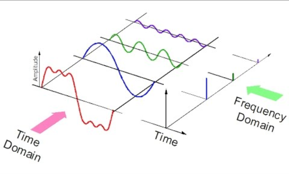
This connection is furthermore empowered by the convolution theorem, which states that this “bridge” preserves the convolution operation:
where the Fourier transform of $f:\mathbb{R}\mapsto\mathbb{R}$ is defined as:
1.3. A frequency basis
Notice that the eigenvectors of the convolution operator are the functions $e_{\omega}:x\mapsto e^{i\omega x}$ since:
Since the Fourier transform is invertible (under certain conditions), with its inverse given by:
we can think of the set of complex exponential, as some basis of the $L_{2}(\mathbb{R})$ space:
Note: The equation above is not rigorous for the continuous case.
However, if we consider finite signals of length $N$
it turns out that it satisfies the same properties than its continuous couterpart, but can additionally provide a true basis for discrete signals:
1.4. From continuous to discrete
As computers are fundamentally limited to discrete representation, we sample real life continuous signals with a certain time period $T$ (the frequency is $1/T$):
Consequently, the higher the period, the closer our discrete representation is from the real signal:
This discrete representation is actually rather convenient, because images are finite and with compact support. It is notably suited for padding zones, wrap, clamp and mirrors.
Without loss of generality, we consider $T=1$ to lighten the equations.
2. Fourier transform of an image
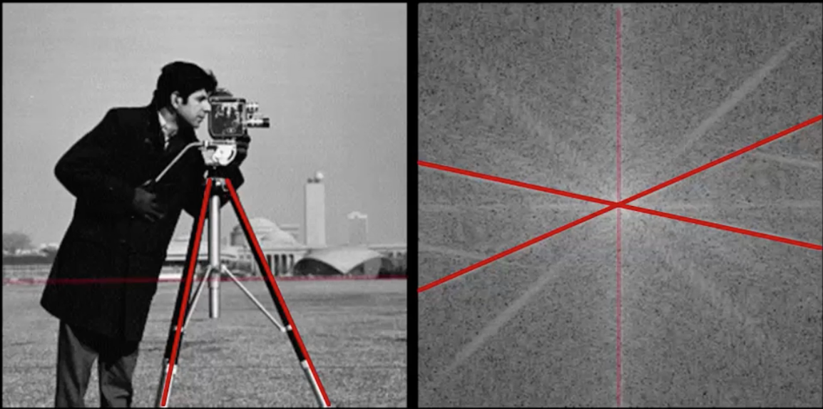
The Fourier Transform is an important image processing tool which is used to decompose an image into its sine and cosine components.
The output of the transformation represents the image in the frequency domain, while the input image is the spatial domain equivalent. In the Fourier domain image, each point represents a particular frequency contained in the spatial domain image:
The Fourier Transform is used in a wide range of applications, such as image analysis, image filtering, image reconstruction and image compression.
2.1. Spatial basis: Dirac delta
In vision computing, Dirac delta helps measure the device’s response to as simple an input as possible (i.e. a pixel):
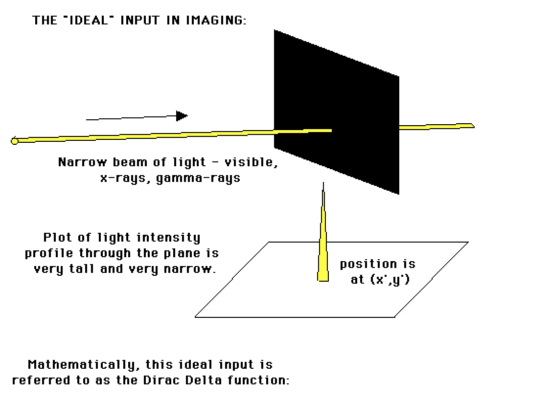
Mathematically, this ideal input is reffered to as the Dirac delta function. It is defined as the limit (in the sense of distributions) of the sequence of zero-centered normal distributions:
Although it can be rigorously defined as a measure (thereby satisfying $\sum_{-\infty}^{\infty}\delta(x)dx=1$), no such function exists. It is nonetheless very useful for approximating functions whose graphical representation is in the shape of a narrow spear:
Basis of $L_{2}(\mathbb{R})$ By convoluting a function $f$ with the Dirac delta function $\delta$, we obtain the function $f$ itself:
Intuitively we can think of the set of Diracs, as the basis of the $L^{2}(\mathbb{R})$ space:
Terminology: We have used $\delta_{y}(x) = \delta(x-y)$
(NOT CLEAR YET FOR THE BASIS - SEE TRANSLATION ALSO)
2.2. 2D Fourier transforms
The 2D Fourier transform is very similar than in the 1D case, excepts there are now two distinct axes on which the integral / sum operate. We define the FT pairs $(F, f)$ as:
and
where $u$ and $v$ are the spatial frequencies. In general complex, we write $F(u, v)$ as:
with:
- Magnitude spectrum: $\mid F(u,v)\mid$ tells you how strong are the harmonics in an image
- Phase angle spectrum: $arctan(\frac{F_{I}}{F_{R}})$ phase spectrum tells where this harmonic lies in space.
2.3. Frequency basis
Just like in the 1D discrete case, we can construct a true frequency basis, composed of “sinusoidal waves” (each with fixed $u, v$):
Note: The term sinusoidal waves is used because the real and imaginary terms are sinusoids on the $x-y$ plane. To get this right, consider the following argument:
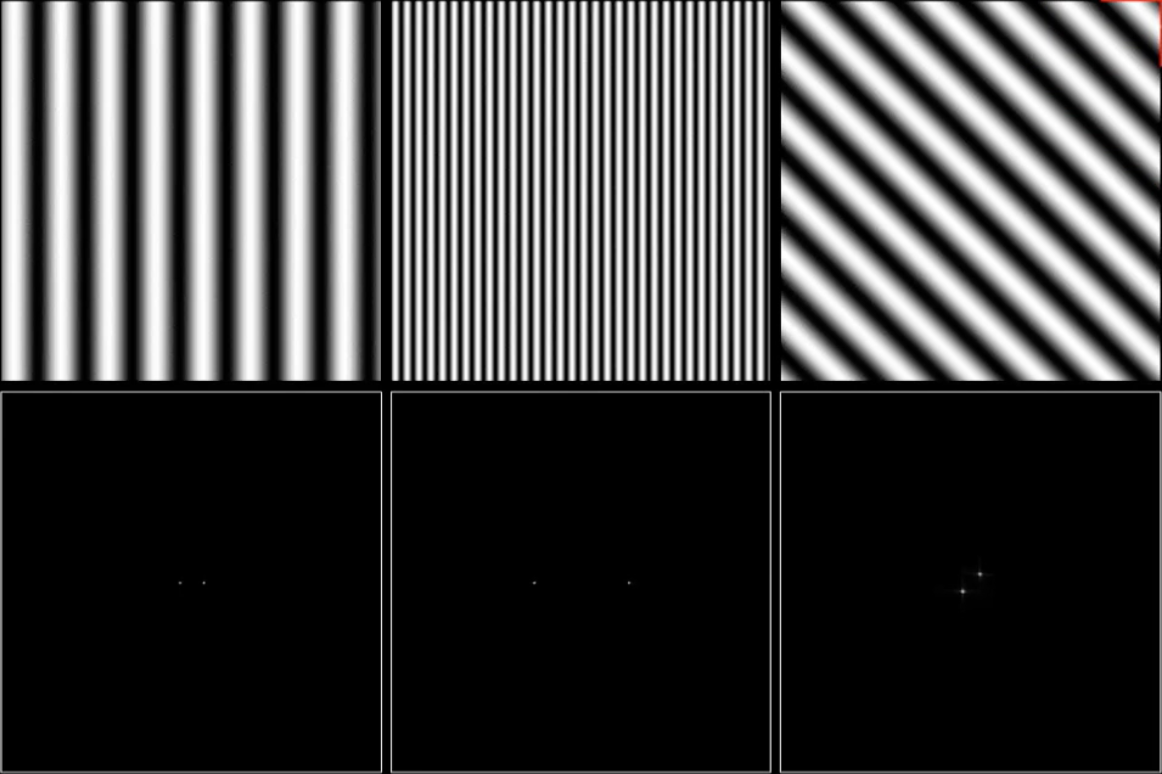
Basis shape? For a given $\textbf{u} = (u, v)$, the maxima $\textbf{x} = (x, y)$ of the real part occur when $2\pi \textbf{u}\cdot \textbf{x} = n\pi$. This imply that the maximas are sets of equally spaced parallel lines with normal $u$ and wave-length $\frac{1}{\sqrt{u^{2} + v^{2}}}$
Meaning: To get some sense of what basis elements look like, we plot some basis element - or rather, their real part - as a function of $x$, $y$ for some fixed $u$, $v$. We get a function that is constant when $(ux+vy)$ is constant. The magnitude of the vector $(u, v)$ gives a frequency, and its direction gives an orientation. The function is a sinusoid with this frequency along the direction, and constant perpendicular to the direction.
3. Sources
- Lecture notes of Maria Vakalopoulou who is doing fantastic research in computer vision at the CVN.
- Difference convolution correlation
- Dirac delta
- Dirac distribution
- Lecture notes
- Lecture notes
- Phase and magnitude
Questions:
- Is the Dirac delta function used today in state of the art?
- Is it a specific case of the Fourier transform?
Laisser un commentaire